Z test
Use case
One sample usage: Estimate how many standard deviation (std) the sample mean is from the population mean.
population: all/entire data.
[John’s score expl] Given mean and std of course score of the entire class, now estimate how good is John’s course score.
Sample mean usage (much more common): If the sample mean is far away enough from the population mean, then we say the sample mean is significantly different from population mean.
[IQ expl] A principal at a certain school claims that the students in his school are above average intelligence. A random sample of thirty students IQ scores have a mean score of 112.5. Is there sufficient evidence to support the principal’s claim? The mean population IQ is 100 with a standard deviation of 15.
- Knows:
- pupulation mean = 100
- population std = 15
- sample size = 30
- sample mean = 112.5
- sample std = ?
- Goal:
- If the sample mean is significant
know population std => Z-test
Limitations
- Know population mean
- Know populatino std
- Population has at least 30 samples (why?)
Methodology
\[Z = \frac{\bar{x}-\mu}{\sigma/\sqrt{n}}\]- \(\bar{x}\): sample mean
- \(\mu\): population mean
- \(\sigma\): population std
- \(n\): sample size
- \(z\): z score.
Note \(\sigma/\sqrt{n}\) is actually the std of the sample mean (not sample std, why). Z score has a standard normal distribution, and when n==1, this simplifies to:
\[Z = \frac{x-\mu}{\sigma}\]Z-test in one-sample case
[John’s score expl]
If we have 40 students taken the final, and course score mean is 75, std is 14, while John got 84, we can compute the z score as
\[z = \frac{84-75}{14} = 0.64\]Here 0.64 means John’s score is 0.64*std higher (because 0.64 is positive) than the mean.
But 0.64*std is not that intuitive to understand, better way is telling me that John is better than x% of students in the class, and this is where z-table can help.
Z-table
Z table uses z score as input and outputs the percentage just as we want in the previous section (area under curve).
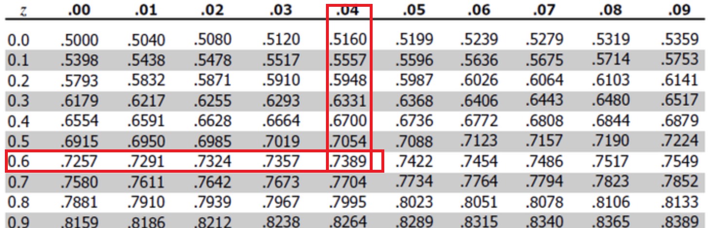
In the example above, by reading the z score table, we know John is better than 0.7389 (73.89%) students in the class (population).
Note we don’t need to know the number of samples in the population in order to use z-table.
Where does z-table come from?
The answer is it is from Gaussian distribution. According to Cental Limite Thereom, if the population is large enough (e.g., more than 30), roughly, the (mean of) course score will follow gaussian distribution, so basically, we are now treating the course score distribution a Gaussian distribution.
\[\frac{1}{\sigma \sqrt{2\pi}} e^{-\frac{(x-\mu)^2}{2\sigma^2}}\]And the CDF (cumulative density function) is:
\[\frac{1}{2}[1+erf(\frac{x-\mu}{\sigma\sqrt{2}})]\]Because when we compute z score we already normalized our input (John’s score), we can just use $\mu=0$ and $\mu=1$, the CDF becomes standard:
\[\frac{1}{2}[1+erf(\frac{x}{\sqrt{2}})]\]Now if we set $x=0.64$, we get
\[\frac{1}{2}[1+erf(\frac{0.64}{\sqrt{2}})] = 0.7389\]This matches the number in z score table.
Z-test in sample mean case
The above [IQ expl]
Population mean \(\mu_0=100\), population std \(\sigma_0=18\), experiment result mean \(\mu = 108\), experiment sample size \(n=30\).
According to z-score equation, we know the z-score is
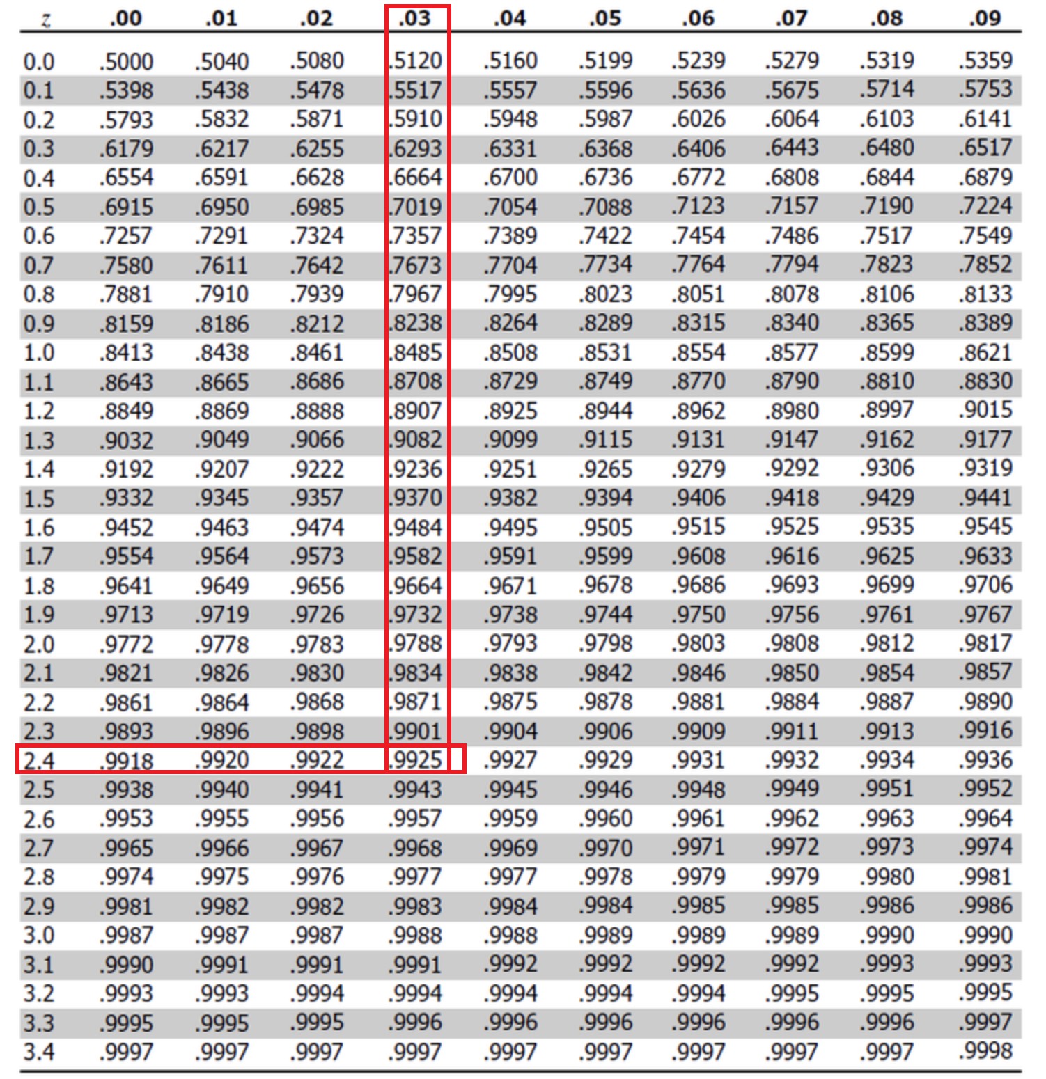
\[Z = \frac{\bar{x}-\mu}{\sigma/\sqrt{n}}\] \[Z = \frac{108 - 100}{18 / \sqrt{30}} = 2.43\]This tells the sample mean is \(2.43\sigma_0\) away from the population mean \(\mu_0\), if you look up z-table, you will know the corresponding area under curve is more than 99.25%.
Well, how do we interprete this 99.25%? Intuitively, this tells us
- Under the null hypothesis, such a result is very unlikely to happen (so far away from the mean). Or,
- Our sample mean is very unlikely to see natually (under the null hypothesis). Or,
- The result rejects the null hypothesis. Or,
- The principal is very likely to be correct, student here indeed have higher IQ (assume the princpal is not cherry-picking clever students from his/her school)
Here, we introduce another concept “reject null hypothesis”, and this is actually all we want to do, we do experiments, design models to find something new, something significantly different from “accepted fact”, don’t we?
But statistics/math do not like “very likely” or “significantly”, we want to define it more accurately, so now we will interprete the result from another perspective to more accurately express our result as “we are xx% (confidence level) sure about the result is correct”.
Confidence level, Alpha (Significance level), P-value, and Confidence Interval
(I don’t know why people invented so many concepts, while actually they are all saying the same thing)
Confidence level
In the [IQ expl], the confidence level (area under curve (AUC)) is 99.25%, it means we are 99.25% sure to reject the null hypotehsis
Alpha
Alpha is the pre-selected threshold we use to reject the null hypothesis.
In real-world scenerio,
- Pre-select an alpha value (say 0.05) before the experiment,
- Find the z-score corresponding to the alpha value (I know, believe me I don’t like this part either), in this case we find the \(z_{\alpha=0.05} = 1.645\),
- Do the experiment, and get our \(z=2.43\),
- \(z > z_{\alpha=0.05}\), it means we are at least 95% confident that the null hypothesis is wrong, so we reject null hypothesis, the result is significant.
P-value
In the [IQ expl], the confidence level is 99.25%, then p-value would be:
\[p = 1 - AUC = 0.0075\]So what is the different between alpha and p-value? Well, they are the same thing, it is just alpha is the pre-selected target, and p-value is the actual result.
In real-world, we often:
- Pre-select an alpha value (say \(z_{\alpha}\) 0.05) before the experiment,
- Do the experiment, and get our \(z=2.43\),
- Check the z-score vs. p-value table, find the p-value \(p=0.007539\),
- \(p < \alpha\), it means the null hypothesis is very unlikely to happen, so we reject null hypothesis, the result is significant.
Confidence Interval (CI)
To compute CI, we need population mean, population std, and sample size, and a pre-selected alpha (or confidence level),
In the [IQ expl], assume we pick alpha=0.05, which correpondes to z=1.96 then the confidence interval is:
\[left = \mu_0 + (\sigma_0/\sqrt(n)) * 1.96 = 100 + (15/\sqrt{30}) * 1.96 = 105.37\] \[right = +\infty\]Which tells us if we want to have at least 95% certainty with current sample size, then our sample mean should lies with \((105.37, \infty)\), our result 108 is in the range, so we can have at least 95% certainty to reject the null hypothesis.
One more example before we continue
[Blood glucose expl] Blood glucose levels for obese patients have a mean of 100 with a standard deviation of 15. A researcher thinks that a diet high in raw cornstarch will have a positive or negative effect on blood glucose levels. A sample of 30 patients who have tried the raw cornstarch diet have a mean glucose level of 102.
Here, the accepted fact is “\(\mu=100\)”, the researcher hypothesizes “\(\mu<100\) or \(\mu>100\) with cornstarch”, so the null hypothesis is “\(\mu=100\) with cornstarch”. And we are computing under the null hypothesis, how likely (probability) the result (\(\mu>=102\) or \(\mu<=98\) over 30 patients, why?) will happen?
- Knows:
- pupulation mean = 100
- population std = 15
- sample size = 30
- sample mean = 102
- sample std = ?
- Goal:
- If the sample mean is significant
know population std => Z-test
\(\mu_0=100\), \(\sigma_0=15\), \(n=30\), \(\mu=140\).
\[z = \frac{102 - 100}{15 / \sqrt{30}} = 0.73\]Looking up in z-score vs. p-value, \(p=0.46539\), so if we choose \(\alpha=0.05\), \(p \gt \alpha\), the null hypothesis is likely to happen (very likely in this case), in other words, the result is not significant.
Larger sample size is always better
But if our sample size is 200, then z=1.88, and p=0.06, which is very close to the target 0.05, intuitively, we are more certain about our result (the sample mean) when we have more samples. This suggests us when we do experiment, we need at least a certain sample size to make sure our result is trustworthy, and the more, the better.
One-side vs Two-side
Note when you look up in the z-score vs. p-value table, it will let you choose “one-side” or “two-side”, what is it?
Actually, in [Blood glucose expl], if you put z=0.73 in the standard Gaussian distribution cdf
\[cdf(z)=\frac{1}{2}[1+erf(\frac{z}{\sqrt{2}})]\]you will get cdf(0.73) = 0.7673, which means p= 1-0.7673 = 0.2327, but this is only one-side p-value, it means
If we randomly choose 30 people (no matter they eat cornstarch or not), we have 23.27% to get a mean blood glucose to be \(\mu_{sample}>=102\).
However, this is not what we want in the [Blood glucose expl], “a diet high in raw cornstarch will have a positive or negative effect on blood glucose levels.” This is telling us we need the two-side p-value, which means
\[\mu_0 - (102-\mu_0) = 100 - (102-100) = 98\]When we see a result (sample mean) = 102, we should interprete it as the blood glucose level should be between 98 and 102, \(98<=\mu_{sample}<=102\). Here 98 is computed from
This means we are looking at a harder problem (more difficult to reject the null hypothesis):
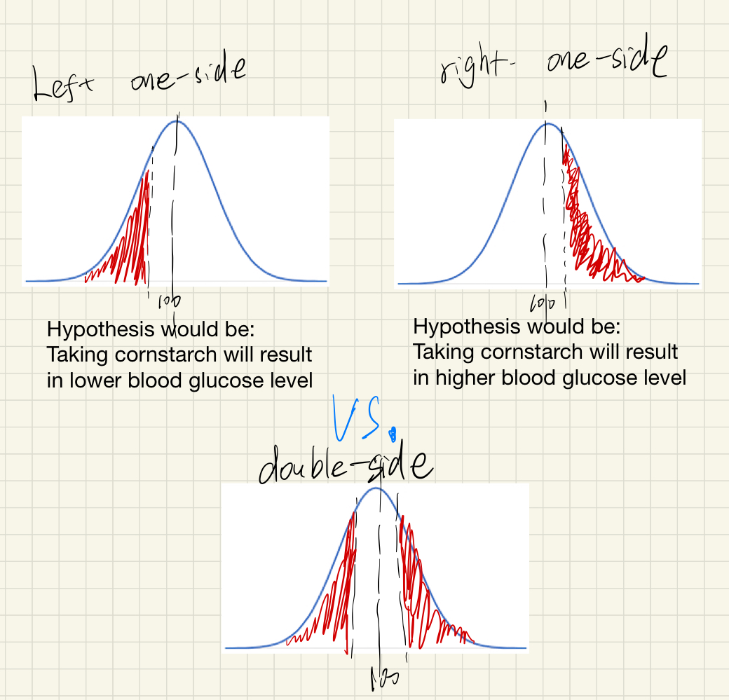
The red area is the probability (p-value) that the result (sample mean) will happen under null hypothesis. We see the probability (p-value) in the two-side case is doubled.
So the p-valud in the [blood glucose expl] is 2 * one-side = 2 * 0.2327 = 0.4654, and since we set our alpha (target value) to be 0.05, \(0.4654 >> 0.05\), we still have a loooong way to go.
What if population std is UNKNOWN?
In reality, even a distribution is Gaussian like, often it’s hard to know population std (population mean is usually easier to acquire/guess, why?), in such cases (i.e., gaussian-like distribution, know population mean, UNKNOWN population std), we would refer to another distribution (student t distribution), which I’ll leave it for the next post.
References
- https://www.wallstreetmojo.com/z-score-formula/